Based on the MLS-C01 exam guideReport an error
MLS-C01· AssociateWeek 7 · Day 1~31 min read
Day 1 - Neural Network Basics: From the Perceptron to Backpropagation
📌 Key Takeaways
- Perceptron = weighted sum + bias + activation. Without a nonlinear activation, no matter how many layers you stack, the network is equivalent to a single linear model.
- The default hidden-layer activation is ReLU; the output depends on the task: binary = Sigmoid / multiclass = Softmax / regression = linear.
- The training loop has four steps: forward pass (prediction) → loss (error) → backpropagation (gradients) → gradient descent (update).
- The problem type decides the loss. Regression = MSE/MAE, binary = BCE, multiclass = categorical cross-entropy. MSE for classification is wrong.
- Epochs, batches, and iterations come up as calculation problems. Iterations per epoch = number of samples ÷ batch size.
When to Reach for Deep Learning
Week 7 covers deep learning, the second pillar of Domain 3 (Modeling). Unstructured data that trees and linear models cannot handle (images, text, audio) and complex nonlinear relationships are deep learning's stage.
| Data shape | First candidate | When to use deep learning | Signals not to use it |
|---|---|---|---|
| Structured (tabular) data | Tree ensembles such as XGBoost | When feature interactions are very complex and data is abundant | "a few thousand rows", "training time limit" |
| Images, video | CNN | Effectively the default choice | Very little data → transfer learning is assumed |
| Sequences (time series, text) | RNN/LSTM/GRU, Transformer | When order and context create meaning | Tabular data where order is meaningless |
| Large-scale language and generation | Transformer family | Assumes using a pretrained model | Options that say to train from scratch |
- MLS-C01 does not ask about deep learning at the level of framework coding. It presents scenarios that assume a conceptual understanding of perceptrons, activations, loss, backpropagation, and hyperparameters.
- Today we get the big picture of how a neural network turns input into predictions and how it learns.
⚠️ Trap: If you memorize "deep learning = always better," you will get a small-tabular-data question wrong. If the data is small and tabular, a tree ensemble is the answer candidate.
The Perceptron: The Smallest Unit of a Neural Network
A perceptron is a single neuron that multiplies inputs by weights, sums them, adds a bias, and passes the result through an activation function.
z = w1*x1 + w2*x2 + ... + wn*xn + b
a = f(z) # f = activation function| Element | Symbol | Role | Is it learned? |
|---|---|---|---|
| Weight | w | Importance of each input | Yes (the core parameter) |
| Bias | b | Shifts the decision boundary in parallel | Yes |
| Activation | f | Injects nonlinearity | No (chosen by the designer) |
- A single perceptron can only do linear separation (it cannot solve XOR).
- This limitation is the motivation for the multilayer perceptron (MLP), which stacks hidden layers.
Without an activation function, no matter how many layers you stack, it is a composition of linear transformations and ends up equivalent to a single linear model. Only with a nonlinear activation can a neural network represent complex, curved decision boundaries. This is the fundamental reason "deep" learning has expressive power.
Hidden Layers and the Multilayer Perceptron (MLP)
If you place one or more hidden layers between the input layer and the output layer, a neural network can approximate nonlinear functions.
Input layer  →  Hidden layer 1  →  Hidden layer 2  →  Output layer
(features)      (low-level         (high-level         (prediction)
patterns) patterns)- The width of a layer (number of neurons) and the depth (number of layers) determine the model capacity.
- The deeper and wider it is, the greater the expressive power, but the greater the risks of overfitting, compute cost, and vanishing gradients.
- Universal approximation theorem: a single-hidden-layer MLP with enough neurons can approximate any continuous function. However, stacking "deeper" often achieves the same expressive power with fewer parameters.
| When you increase model capacity | What you gain | What you lose |
|---|---|---|
| Deeper layers | Hierarchical abstraction, parameter efficiency | Vanishing gradients, unstable training |
| Wider layers | More diverse patterns in the same layer | Parameter explosion, overfitting, memory |
Activation Functions
The key element that injects nonlinearity between layers. The exam asks "what to use where."
| Function | Output range | Main use | Vanishing gradient | Caveat |
|---|---|---|---|---|
| Sigmoid | (0, 1) | Binary classification output | Severe at both ends | Output is not zero-centered |
| Tanh | (-1, 1) | Hidden layers (legacy) | Present at both ends | Zero-centered, so training is more stable than Sigmoid |
| ReLU | [0, ∞) | Default for hidden layers | None in the positive region | "Dead ReLU" on negative inputs |
| Leaky ReLU | (-∞, ∞) | When ReLU dies | None | Keeps a small negative slope to keep the neuron alive |
| Softmax | (0,1), sums to 1 | Multiclass classification output | — | Produces a probability distribution over classes |
| Linear (none) | (-∞, ∞) | Regression output | — | If used in a hidden layer, nonlinearity disappears |
# Conceptual definitions
relu(z)    = max(0, z)
sigmoid(z) = 1 / (1 + exp(-z))
softmax(z_i) = exp(z_i) / sum(exp(z_j) for all j)
Selection guide:
- Hidden layers: The default is ReLU (or variants such as Leaky ReLU and GELU). It is resistant to vanishing gradients and fast.
- Binary classification output: Sigmoid with 1 node.
- Multiclass classification output: Softmax (as many nodes as classes).
- Regression output: Linear with no activation (or a function that fits the output range).
When the input is large or small, the derivatives of Sigmoid/Tanh approach 0, so the gradient keeps shrinking during backpropagation, causing the vanishing gradient problem. ReLU keeps the gradient constant at 1 in the positive region and greatly eases this problem, but because it always outputs 0 for negative inputs, some neurons can become permanently inactive ("dead ReLU"), and Leaky ReLU appeared to prevent this.
⚠️ Trap: In options asking about the output-layer activation, ReLU and Tanh get mixed in. These two are for hidden layers. If you need probabilities, use Sigmoid/Softmax; for continuous values, use linear.
Forward Pass and Loss
Training happens through flows in two directions. First, the forward pass produces a prediction.
Input → repeat (weighted sum + activation) at each layer → final prediction ŷThe difference between the prediction ŷ and the actual answer y is quantified by the loss function (loss).
Loss Function Selection Table
| Problem type | Output layer | Loss function | Why |
|---|---|---|---|
| Regression | Linear (no activation) | MSE (mean squared error) | Penalizes large errors heavily |
| Regression (many outliers) | Linear | MAE (absolute error) | Less affected by outliers |
| Binary classification | Sigmoid, 1 node | Binary cross-entropy (BCE) | Log loss of probability predictions |
| Multiclass (mutually exclusive) | Softmax, K nodes | Categorical cross-entropy | Compares probability distributions |
| Multilabel (can co-occur) | Sigmoid, K nodes | Sum of per-label BCE | Classes are not mutually exclusive |
- Using MSE for classification makes training slow and unstable, so cross-entropy is the standard.
- The smaller the loss, the better the model. The goal of training is to find "the weights that minimize the loss."
The loss is the optimization target, while the evaluation metric is the business decision criterion. If a question asks "which metric should be used to choose a model" and you pick the training loss, it is wrong.
Loss and Evaluation Metrics Are Different — Metric Interpretation Table
| Metric | Calculation | What a high value means | When to prioritize | Trap |
|---|---|---|---|---|
| Accuracy | (TP+TN)/total | Often right overall | Only when classes are balanced | If imbalanced, 99%+ even with "all negative" |
| Precision | TP/(TP+FP) | Few false positives | False positives are costly | Easily raised by predicting positive for only a few |
| Recall | TP/(TP+FN) | Few misses | Misses are costly (fraud, disease) | 1.0 if you predict everything positive |
| F1 | Harmonic mean of precision and recall | A good balance of both | When the two costs are similar | Hides which side is the problem |
| ROC-AUC | Area under the TPR-FPR curve | Discrimination independent of threshold | Threshold undecided, comparing models | Optimistic under extreme imbalance |
| PR-AUC | Area under the precision-recall curve | Discrimination for the minority class | When the positive rate is extremely low | The value also changes when the class ratio changes |
| RMSE | Square root of the mean squared error | Few large errors | Regression, when large errors should be penalized heavily | Sensitive to outliers |
| MAE | Mean of absolute errors | Small average error | Regression, when robustness to outliers is needed | Treats large errors leniently |
Accuracy is meaningless on imbalanced data. If positives are 1%, just predicting "all negative" gives 99%. If the question says "positive cases are very rare," discard the accuracy option first and look at recall and PR-AUC.
Backpropagation
To reduce the loss, you need to know how much each weight contributes to it. Backpropagation computes the gradient of the loss by propagating it from the output layer toward the input layer using the chain rule.
1. Forward pass: compute the prediction ŷ
2. Compute the loss: L(ŷ, y)
3. Backpropagation: compute ∂L/∂w from output to input using the chain rule
4. Update the weights: w ← w - η * ∂L/∂w   (η = learning rate)
5. Repeat 1~4 per batch/epoch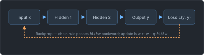
- The gradient tells you "if I increase this weight, in which direction and by how much does the loss change."
- With gradient descent, the weights are moved a little at a time in the direction opposite to the gradient.
- This process is repeated tens of thousands to hundreds of thousands of times in batches of data to lower the loss.
Backpropagation is paired with the optimizer (Day 4). Backpropagation computes "in which direction," and the optimizer decides "how much and how" to move.
As layers get deeper, the product of derivatives in the chain rule gets longer. If each term is less than 1, the product converges to 0, causing a vanishing gradient; if greater than 1, it diverges, causing an exploding gradient. That is why deep networks combine activation choice (ReLU), normalization (batch normalization), and structural shortcuts (residual connections).
Epoch, Batch, Iteration
| Term | Meaning |
|---|---|
| Epoch | One full pass through all the training data |
| Batch | A group of samples used for a single weight update |
| Batch size | Number of samples in one batch (memory vs stability trade-off) |
| Iteration | Processing one batch = one weight update |
- Example: with 1000 samples and a batch size of 100, one epoch = 10 iterations.
- Formulas:
iterations per epoch = number of samples ÷ batch size,total updates = iterations per epoch × number of epochs.
Batch Size Trade-offs
| Batch size | Gradient estimate | Memory/GPU | Generalization tendency | Typical situation |
|---|---|---|---|---|
| Large | Stable (less noise) | Uses a lot, high GPU utilization | May get slightly worse | Large-scale GPUs, goal is fast throughput |
| Small | Noisy | Uses little | Sometimes helps escape local minima | Out of memory (OOM), small data |
A large batch size gives a stable gradient estimate and high GPU utilization, but uses a lot of memory and may slightly worsen generalization. A small one mixes in noise, which sometimes helps escape local minima. On the exam, if "training fails due to out of memory (OOM)," reducing the batch size is the first-line remedy.
Symptom → Cause → Remedy
| Symptom | Cause | First-line remedy |
|---|---|---|
| Loss is NaN/explodes | Learning rate too high, exploding gradients | Lower the learning rate |
| Convergence is very slow | Learning rate too low | Raise the learning rate or use scheduling, adaptive optimizers |
| Making the network deeper made it worse | Vanishing gradients | ReLU family, batch normalization, residual (skip) connections |
| Training loss↓ validation loss↑ | Overfitting | Dropout, regularization, augmentation, early stopping |
| Both losses are high | Underfitting | Increase model capacity, train longer, enrich features |
| Training stops with OOM | Batch or model too large | Reduce batch size |
| Hidden-layer output stays at 0 | Dead ReLU | Replace with Leaky ReLU, etc. |
When Training Neural Networks on AWS
| Situation | Choice | Reason |
|---|---|---|
| You want to run your own TensorFlow/PyTorch training script | SageMaker Script Mode | Runs your code as-is in a managed training container |
| You don't want to build per-framework-version environments yourself | Deep Learning Containers (DLC) | Prebuilt managed images |
| Searching hyperparameters such as learning rate and batch size | Automatic Model Tuning | Efficient search through Bayesian optimization |
| Deep learning training that needs GPUs | ml.p / ml.g instance families | For GPU-accelerated training |
| Starting quickly from a pretrained model | SageMaker JumpStart | Provides pretrained models and fine-tuning scripts |
In the next note, we cover the CNN (convolutional neural network), which redesigns this neural network for images, and the distinctions among computer vision tasks.
📖 Glossary
- Perceptron: The smallest-unit neuron of a neural network, which adds a bias to the weighted sum of inputs and passes it through an activation.
- Weight / bias: Parameters adjusted by training. The weight is the importance of an input, and the bias shifts the decision boundary in parallel.
- Activation function: A function that injects nonlinearity between layers. Without it, even a deep network is the same as a linear model.
- Vanishing gradient: A phenomenon where the product of derivatives in backpropagation converges to 0, so the earlier layers do not learn.
- Dead ReLU: A neuron that receives only negative inputs and always outputs 0. Its gradient is 0, so it never revives.
- Forward pass: The computation in the direction that passes the input through each layer to produce a prediction.
- Backpropagation: An algorithm that computes the gradient of the loss by propagating it from output to input using the chain rule.
- Loss function: A single number summarizing the difference between predictions and answers. The target that training tries to minimize.
- Cross-entropy: A loss for probability predictions. Binary uses BCE, and multiclass uses categorical cross-entropy.
- Epoch / batch / iteration: One pass over all the data / the group used for one update / processing one batch (= one update).
📝 Practice Questions
Click a choice to reveal the answer and explanation.
Question 1
Which is the MOST appropriate output layer activation function for a multiclass (10-class) image classification neural network?
Question 2
What is the main reason training goes poorly when using Sigmoid in the hidden layers of a deep neural network, and what is the usual remedy?
Question 3
What is the representational power of a multilayer neural network with no activation functions at all (only linear)?
Question 4
When training for 5 epochs with 8,000 samples and a batch size of 200, what is the total number of weight updates (iterations)?
Question 5
Which BEST describes the role of backpropagation?