Based on the MLS-C01 exam guideReport an error
MLS-C01· AssociateWeek 7 · Day 2~31 min read
Day 2 - CNN: Convolutional Neural Networks and Computer Vision
📌 Key Takeaways
- A CNN processes images efficiently thanks to three ideas: local receptive fields + weight sharing + translation invariance.
- Convolution extracts patterns and pooling shrinks the size. Pooling has no learnable parameters.
- You must clearly distinguish classification (labels) / object detection (boxes + classes) / semantic segmentation (pixels).
- ResNet's residual (skip) connections are the fix for the problem that networks of 100+ layers would not train.
- SageMaker provides the Image Classification, Object Detection, and Semantic Segmentation built-ins plus Ground Truth labeling.
Why Convolution, Not Fully Connected?
Images and video have an enormous number of pixels. Feeding them straight into a fully connected (Dense) neural network makes the parameter count explode, and the network also fails to learn translation invariance. A convolutional neural network (CNN) solves this by sliding small filters across the whole image to extract local patterns.
- A 224×224×3 color image flattened into a Dense layer gives roughly 150,000 input nodes.
- If the first hidden layer has 1,000 nodes, that is 150 million weights — an explosion.
| Aspect | Fully connected (Dense) | Convolution (CNN) |
|---|---|---|
| Range one neuron sees | The whole image | A small local region (receptive field) |
| Parameters | Blow up in proportion to input size | Fixed at filter size × number of filters |
| An object that moved | Treated as a different input | The same filter still detects it |
| Training data required | Large | Relatively small |
The three ideas a CNN uses:
- Local receptive field: one neuron sees only a small region, not the whole image.
- Weight sharing: the same filter is reused at every position, which collapses the parameter count.
- Translation invariance: a cat is detected with the same filter wherever it is.
Weight sharing rests on the assumption that "a filter that finds a cat's ear works exactly the same way at any position in the image." This assumption reduces the parameters to learn and lets the model generalize well even on limited data. It builds the property "the meaning of an image is preserved under spatial shifts" into the structure itself as an inductive bias.
MLS-C01 does not ask about the internal math of CNNs. It asks about the roles of convolution and pooling, image classification vs object detection, and choosing SageMaker built-ins and architectures.
Convolution Layer
A small filter (kernel) slides over the input and a dot product is computed at each position, producing a feature map.
Input image  *  Filter (e.g., 3x3)  →  Feature map
(emphasizes edges, texture, shape patterns)
Convolution Hyperparameter Table
| Hyperparameter | What it determines | Effect on the output | Rule of thumb |
|---|---|---|---|
| Number of filters | How many kinds of patterns to detect | The output channel count equals the number of filters | Usually increased as the network gets deeper |
| Kernel size | Region seen at once (3×3, 5×5, etc.) | Larger shrinks the output more and costs more compute | Smaller captures finer detail |
| Stride | Step size of the filter | Larger gives a smaller output | Acts as downsampling |
| Padding | Whether to pad the edges with 0s | same = keep the size, valid = shrink | Use same to preserve size |
Stride 1 + same padding           Stride 2
┌───────────┐                    ┌───────────┐
│ ▢▢▢▢▢▢▢▢ │ → size preserved    │ ▢▢▢▢▢▢▢▢ │ → shrinks to half size
└───────────┘                    └───────────┘
Abstraction deepens as layers are stacked: low level (edges) → mid level (texture, parts) → high level (whole objects).
One side of the output is determined by the four hyperparameters:
output size = floor( (input size + 2×padding − kernel size) / stride ) + 1
output channels = number of filters
As layers stack up, the region of the original image that one neuron sees (its receptive field) grows. A single 3×3 filter sees only 3×3, but stacking another 3×3 on top makes it see 5×5 relative to the original. That is why a VGG-style design that stacks small kernels deeply can see a wide region with fewer parameters than one large kernel. Pooling and large strides make this expansion even faster.
- If the question says "we want to keep the output size unchanged," the answer is
samepadding. Increasing the stride or choosingvalidpadding shrinks the size.
Pooling Layer
Pooling reduces the spatial size of the feature map, lowering computation and making the model robust to small position changes.
| Type | Operation | Characteristic |
|---|---|---|
| Max Pooling | Maximum within the region | Preserves the strongest features, most common |
| Average Pooling | Average within the region | Smooth downsampling |
| Global Average Pooling | Average over each whole channel | Replaces Dense and reduces parameters |
- Pooling has no learnable parameters (it is a fixed operation).
- Downsampling widens the receptive field and reduces overfitting.
⚠️ Trap: An option saying "pooling adds weights to raise expressiveness" is wrong. Adding weights is the role of convolution and Dense layers.
Typical CNN Architecture
[Conv → ReLU → Pool] × N  →  Flatten/GAP  →  Dense  →  Softmax
   Feature extraction (backbone)            Classification head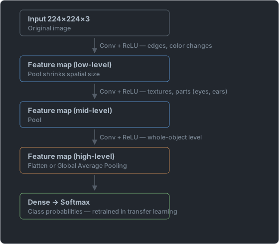
- The front part (conv/pool blocks) is the feature extractor (backbone).
- The back part (Dense + Softmax) is the classification head.
- Transfer learning (Day 4) often reuses the backbone and trains only the head.
| Block | What it does | Learnable parameters | In transfer learning |
|---|---|---|---|
| Conv | Extracts local patterns | Yes (filter weights) | Usually reused (frozen) |
| ReLU | Injects nonlinearity | None | — |
| Pool | Spatial reduction, robustness | None | — |
| Flatten / GAP | Turns the 2D feature map into a vector | None | GAP is better for saving parameters |
| Dense + Softmax | Decides the class | Yes | Usually replaced and retrained |
- Flatten spreads the entire feature map into the Dense layer, so parameters surge. In a question saying "the fully connected layer has too many parameters," replacing it with Global Average Pooling is the right direction.
Representative Architectures
Knowing the names and core ideas gives you clues in the question stem.
| Architecture | Key idea |
|---|---|
| LeNet | Early CNN (handwritten digit recognition) |
| AlexNet | Revived deep learning with ReLU, dropout, and GPUs (2012) |
| VGG | Simple, regular structure that stacks 3×3 filters deeply |
| ResNet | Residual (skip) connections make training of very deep networks possible |
| Inception | Combines multiple kernel sizes in parallel |
There was a paradox where making a network deeper actually made training worse (vanishing gradients). ResNet's residual/skip connection adds the input directly to the output (H(x)=F(x)+x), creating a shortcut for gradients to flow, so networks of 100+ layers train stably. The exam asks about it as the fix for "a deep network fails to train."
Image Classification vs Object Detection vs Segmentation
Distinguishing the CNN applications precisely is the heart of the exam.
| Task | Output | Question it answers | Representative algorithms | SageMaker built-in |
|---|---|---|---|---|
| Image classification | 1 label (or several) per image | "What is this picture?" | General CNNs such as ResNet, VGG | Image Classification |
| Object detection | Class + bounding box for multiple objects | "Where, what, and how many?" | SSD, YOLO, Faster R-CNN | Object Detection |
| Semantic segmentation | Class per pixel | "Which object is each pixel?" | U-Net, FCN | Semantic Segmentation |
⚠️ Trap: "How many are where" is detection; "separate regions pixel by pixel" is segmentation. A single verb in the stem ("count/locate" vs "pixel-level") decides the answer.
SageMaker Built-ins and Data Formats
- Image Classification: single- or multi-label classification. ResNet-based. Supports a transfer learning mode.
- Object Detection: SSD-based. Outputs boxes + classes.
- Semantic Segmentation: pixel-level classification.
- Input is usually RecordIO (recommended, fast) or image files + annotations. For large data, use Pipe mode streaming.
- Labeling: SageMaker Ground Truth (provides task templates for bounding boxes and segmentation).
Situation → AWS Choice Mapping Table
| Situation | Choice | Why |
|---|---|---|
| Attach one category to each photo | Image Classification | The standard built-in for classification tasks |
| Count and locate people and vehicles from store CCTV | Object Detection | Needs box + class output |
| Separate building regions at pixel level in satellite images | Semantic Segmentation | Needs a class per pixel |
| No ground-truth bounding boxes | Ground Truth | Provides labeling task templates and a workforce |
| Training data is several TB and cannot fit on disk | Pipe mode + RecordIO | Streams input from S3 |
| Start quickly from pretrained weights | Transfer learning mode / JumpStart | Little data, short time |
When Data Is Scarce: Augmentation and Transfer Learning
| Technique | Effect | When | Caution |
|---|---|---|---|
| Rotation / flip | Gains orientation diversity | Objects whose orientation does not matter | Flipping letters or digits breaks their meaning |
| Random crop | Gains position and scale diversity | Most classification tasks | Make sure the target is not cropped out |
| Color jitter | Robust to lighting changes | When lighting conditions vary | Avoid if the color itself is the label |
| Transfer learning (pretrained weights) | High generalization with little data | First choice when data is scarce | Gain shrinks if the domain is too different |
When images are scarce, data augmentation (rotation, flipping, cropping, color jitter) increases training diversity and reduces overfitting. SageMaker Image Classification and Object Detection have augmentation options built in. Also, transfer learning with ImageNet-pretrained weights performs better and takes less time than training from scratch on little data (linked to Day 4).
Apply augmentation to the training set only. Augmenting the validation or test set distorts the evaluation.
Reading Classification Performance — Metric Interpretation Table
Image classification is still classification. When classes are skewed, accuracy misleads people.
| Metric | What it tells you | When to prioritize | Trap |
|---|---|---|---|
| Accuracy | Share of all predictions that were right | Only when classes are balanced | In a 1% defect-rate inspection, "everything is normal" is also 99% |
| Precision | Of those called positive, how many are truly positive | False-positive cost is high (scrapping good products) | Easy to raise by predicting positive for only a few |
| Recall | Share of actual positives caught | False-negative cost is high (shipping defective products) | Predicting everything positive gives 1.0 |
| F1 | Balance of precision and recall | When the two costs are similar | Hides which side is the problem |
| ROC-AUC | Discrimination independent of threshold | Comparing models | Optimistic under extreme imbalance |
| PR-AUC | Discrimination for the minority class | When defects are very rare | Value changes if the class ratio changes |
Question Clue → Answer Mapping
| If the question says this | It points to |
|---|---|
| "We want to know which category each image belongs to" | Image classification |
| "How many are where," "location and count" | Object detection (SSD/YOLO) |
| "At pixel level," "separate regions precisely" | Semantic segmentation (U-Net/FCN) |
| "There is no label data," "annotation work is needed" | Ground Truth |
| "Only a few hundred training images" | Transfer learning + data augmentation |
| "Making the network deeper made training fail" | ResNet (residual connections) |
| "The input data is too large and loading is slow" | RecordIO + Pipe mode |
| "The fully connected layer has too many parameters" | Global Average Pooling |
If you see only "improve accuracy" and automatically pick a deeper architecture, you will be wrong. When there is also a clue that data is scarce, the answer is not a bigger structure but transfer learning and augmentation.
Symptom → Cause → Remedy
| Symptom | Cause | First remedy |
|---|---|---|
| Only training accuracy is high, validation is low | Insufficient data → overfitting | Data augmentation + transfer learning |
| Training got worse after stacking more layers | Vanishing gradients | Residual (skip) connections (ResNet family) |
| GPU out of memory (OOM) | Batch size or image resolution too large | Reduce batch size, adjust input resolution |
| Cannot get object locations | Wrong task type chosen (solving it as classification) | Switch to object detection |
| Training data loading is the bottleneck | File-by-file I/O | RecordIO + Pipe mode |
| Dense head has too many parameters | Flatten wired directly in | Replace with Global Average Pooling |
The next post covers data where order, not space, creates meaning — RNN, LSTM, GRU, and the Transformer.
📖 Glossary
- Convolution: an operation that slides a small filter over the input and computes dot products to extract local patterns.
- Filter (kernel) / feature map: the small grid of weights a convolution learns / the output produced by passing the input through that filter. One channel is created per filter.
- Stride / padding: the step size of the filter / a setting that pads the edges with 0s to control the output size.
- Local receptive field: the small range of input one neuron sees. It widens as layers get deeper.
- Weight sharing: reusing the same filter at every position in the image. Parameters shrink greatly.
- Translation invariance: the property that an object is still detected with the same filter even if it moves within the image.
- Pooling: an operation that shrinks the feature map using the maximum or average of a region. It has no learnable parameters.
- Residual (skip) connection: a structure that adds the input directly to the output, creating a shortcut for gradients to flow. The core of ResNet.
- Backbone / head: the front part that extracts features / the back part that produces the final prediction. Transfer learning usually reuses the backbone.
- RecordIO: the input format SageMaker recommends, which bundles many images to favor sequential reads. It is used together with the bounding-box annotations that object detection outputs.
📝 Practice Questions
Click a choice to reveal the answer and explanation.
Question 1
You need to know "how many vehicles and pedestrians are in the photo and where they are located." Which task type is MOST appropriate?
Question 2
Which of the following is NOT a role of the pooling layer in a CNN?
Question 3
Which representative architecture introduced residual (skip) connections so that networks can be trained stably even when stacked more than 100 layers deep?
Question 4
What is the key reason a CNN is advantageous for images compared with a fully connected (Dense) neural network?
Question 5
When image training data is very scarce, what is the MOST appropriate first remedy for reducing overfitting?