Based on the MLA-C01 exam guideReport an error
MLA-C01· AssociateWeek 2 · Day 3~27 min read
Day 3 - Query & Exploration: Athena, Redshift, EDA Basics
📌 Key Takeaways
- Athena queries S3 directly with serverless SQL. Billing is by data scanned ($5/TB) — cutting scan volume is cutting cost.
- Athena's three big cost levers: columnar format (Parquet) + partitioning + compression.
- Redshift is a load-based data warehouse (MPP). It is strong at repeated high-performance BI. Spectrum is the bridge to S3.
- Redshift ML trains and runs inference with
CREATE MODELSQL without moving the data. - Before modeling, always check distributions, missing values, outliers, correlations, class imbalance, and data leakage with EDA.
Amazon Athena: Querying S3 with SQL
Once you have ingested and cataloged the data, it is time to read and understand it. Before building a model, a data scientist always looks into the data — this is EDA (Exploratory Data Analysis).
Athena is a service that queries data stored in S3 with serverless SQL. It is based on the Presto/Trino engine and has no cluster provisioning at all. It uses the table definitions in the Glue Data Catalog as they are.
- Serverless: No infrastructure to manage. It runs only when you query.
- schema-on-read: Query the data while leaving it in S3, without moving it.
- Billing = data scanned: Charged per byte the query scans ($5/TB). Minimizing scan volume is cost savings.
-- Query a table registered in the Glue Catalog directly
SELECT customer_id, AVG(amount) AS avg_amount
FROM ml_datalake.transactions
WHERE year = '2026' AND month = '06'   -- partition filter reduces scan volume
GROUP BY customer_id
ORDER BY avg_amount DESC
LIMIT 100;
In the query above, WHERE year='2026' AND month='06' triggers partition pruning, so only the Parquet files of the matching partition are scanned.
The three big levers for reducing scan volume
| Lever | Principle | Effect |
|---|---|---|
| Columnar format (Parquet/ORC) | Reads only the needed column blocks | Reduced by the ratio of columns |
| Partitioning | Reads only the folders matching the condition | Reduced by the ratio of partitions |
| Compression (Snappy/GZIP) | The physical bytes themselves get smaller | 2–10x reduction |
The three levers multiply. That is why a well-designed Parquet query becomes dozens of times cheaper than a full CSV scan.
The fact that Athena cost is proportional to the "data scanned" directly affects ML data preparation. A full CSV scan is expensive and slow, but on well-partitioned Parquet the same query runs at a much lower cost. If you frequently run queries that extract ML features, this difference accumulates.
Athena suits quick feature exploration in an ML workflow. Before SageMaker reads Parquet from S3 as training data, an analyst checks with SQL in Athena "what is the target distribution? is there class imbalance?" You can also use Athena CTAS (CREATE TABLE AS SELECT) to save query results to S3 as Parquet and build a training dataset directly.
-- Create a training dataset as Parquet with CTAS
CREATE TABLE ml_datalake.churn_training
WITH (format = 'PARQUET', external_location = 's3://ml-datalake/curated/churn/')
AS
SELECT customer_id, tenure, monthly_charges, churned
FROM ml_datalake.transactions
WHERE year = '2026';
Amazon Redshift: Data Warehouse
Redshift is a petabyte-scale data warehouse (OLAP). It loads data into Redshift's internal nodes (or Redshift Serverless) and processes complex analytical queries at high speed with MPP (Massively Parallel Processing).
| Aspect | Athena | Redshift |
|---|---|---|
| Model | Serverless, queries S3 directly | Data warehouse (loading required) |
| Data location | S3 (no movement) | Inside the cluster (or Serverless) |
| Suited for | Ad hoc/occasional queries, exploration | Repeated high-performance analytics, BI dashboards |
| Billing | Scan volume | Cluster (node hours) or RPU |
| Preparation work | None (catalog only) | Loading (COPY), designing distribution keys and sort keys |
| Answer keywords | "occasional", "minimal management overhead", "leave in S3 as is" | "repeated BI", "complex joins", "sustained workload" |
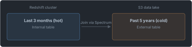
Redshift Spectrum is the bridge between the two — from Redshift you can query data in S3 directly as external tables. Keep frequently used (hot) data inside Redshift and cold data in S3, and join them with Spectrum.
On the ML integration side there is also Redshift ML. With the SQL CREATE MODEL statement you can call SageMaker Autopilot from inside Redshift to train and run inference. You create a prediction column with SQL alone, without moving the data.
-- Redshift ML: train a model with SQL (internally calls SageMaker Autopilot)
CREATE MODEL churn_predictor
FROM (SELECT tenure, monthly_charges, churned FROM transactions)
TARGET churned
FUNCTION predict_churn
IAM_ROLE 'arn:aws:iam::123456789012:role/RedshiftMLRole'
SETTINGS (S3_BUCKET 'ml-datalake-redshiftml');
An easy-to-confuse comparison — "ad hoc exploration/occasional queries + minimal management overhead + leave the data in S3" means Athena. "Repeated high-performance BI queries + complex joins + sustained workload" means Redshift. "Joining cold S3 data from Redshift" means Redshift Spectrum. "ML with SQL without moving data" means Redshift ML.
EDA (Exploratory Data Analysis) Basics
Now that you can query the data, it is time to understand it. EDA is the process of grasping the structure, quality, and relationships of the data before modeling, and it provides the basis for feature engineering and data cleansing.
| Check | Question | Response when found |
|---|---|---|
| Distribution | How is each feature distributed? | Skew → log transform |
| Missing values | Which columns have many missing values? | Imputation or removal |
| Outliers | Are there extreme values? | Clipping, removal, robust scaling |
| Correlation | What are the correlations between features and with the target? | Remove multicollinearity, drop meaningless features |
| Class imbalance | Is the target distribution skewed? | Over/under-sampling, class weight |
| Cardinality | How many unique values do categorical columns have? | Decide the encoding strategy |
| Data leakage | Is there an unrealistically high correlation with the target? | Remove that feature |
import pandas as pd

df = pd.read_parquet("s3://ml-datalake/curated/churn/train.parquet")

# Basic statistics
print(df.describe())          # numeric distributions (mean/std/quartiles)
print(df.isnull().mean())     # missing ratio per column
print(df["churned"].value_counts(normalize=True))  # check class imbalance
print(df.corr(numeric_only=True))  # feature correlation matrix
How to read correlation coefficients — a table that leads straight to judgments in EDA.
| Observation | What it means | Action |
|---|---|---|
| Feature-target correlation ≈ 0 | Contributes nothing to prediction | Drop candidate |
| Feature-target correlation 0.99 | Suspected data leakage | Trace the cause, then remove |
| Feature-feature correlation 0.95 | Multicollinearity | Keep only one or reduce dimensions |
| Missing rate > 50% | Almost no information | Remove the column or turn it into a "was missing" flag |
| Minority class < 1% | Extreme imbalance | Stratified split + resampling + PR-AUC |
EDA is a concept established in 1977 by the statistician John Tukey in his book Exploratory Data Analysis. The core philosophy is "before forming and testing hypotheses, first let the data speak for itself." Visualizations such as box plots, histograms, and scatter plots are also Tukey's legacy. If you skip EDA in ML, you miss class imbalance or data leakage and the model learns wrong patterns.
⚠️ Trap: The most dangerous mistake at the EDA stage is data leakage. For example, if a column named "payment completion date" effectively contains the "did purchase" target in advance, validation accuracy is 99% but it is useless in actual deployment. If EDA shows a feature with an unrealistically high correlation (e.g., 0.99) with the target, suspect leakage.
The environment for doing EDA on AWS is usually SageMaker Studio / notebooks. In a notebook you query with SQL through Athena, or read Parquet in S3 directly with pandas to analyze it. For large-scale data, SageMaker Data Wrangler offers visual EDA and transformation bundled together (covered in depth in Week 3).
[S3 Parquet] ──┬──> Athena SQL (large-scale aggregation and sampling)
               ├──> pandas notebook (detailed analysis and visualization)
               └──> Data Wrangler (visual EDA + transformation + quality report)
Tool Selection Summary
| Requirement | Answer |
|---|---|
| Occasional SQL exploration of S3 data, minimal management overhead | Athena |
| Athena cost is high | Parquet + partitioning + compression, no SELECT * |
| Repeated high-performance BI, complex joins | Redshift |
| Hot data in the cluster, cold in S3, join them | Redshift Spectrum |
| ML with SQL alone, without moving data | Redshift ML |
| Save query results as a training dataset (Parquet) | Athena CTAS |
Habits That Make Athena Queries Fast and Cheap
The constraint of scan-based billing even changes how you write queries.
| Habit | Bad example | Good example |
|---|---|---|
| Column selection | SELECT * | Name only the columns you need |
| Partition filter | Query everything with no condition | WHERE year='2026' AND month='06' |
| Previewing | Sort everything and then look | LIMIT together with a partition filter |
| Repeated aggregation | Run the same heavy query every time | Create an intermediate table with CTAS and reuse it |
| Joins | Join large tables blindly | Reduce them first with filters and aggregation, then join |
LIMITalone may not reduce scan volume. Partition pruning must also apply for it to actually read less.- A Parquet intermediate table made with CTAS is used both for later repeated queries and for creating training datasets.
Design Decisions That Come with Choosing Redshift
Unlike Athena, Redshift is "load-based," so the data placement design governs performance.
| Decision | What you determine | If done wrong |
|---|---|---|
| Distribution style (DISTKEY) | How rows are scattered across nodes | Data moves between nodes on every join |
| Sort key (SORTKEY) | Sort order within blocks | Range queries read unnecessary blocks too |
| Compression encoding | Per-column storage method | Storage size and I/O grow |
| Load method | Parallel load with COPY | Row-by-row INSERT is very slow |
This design burden is the practical basis for the rule "Athena for occasional exploration, Redshift for repeated high-performance analytics."
What to Plot in EDA
| Visualization | What it checks | Follow-up action |
|---|---|---|
| Histogram | Distribution shape, skew | Whether to apply a log transform |
| Box plot | Quartiles and outliers | Outlier handling by the IQR rule |
| Scatter plot | Relationship between two variables | Derived features if the relationship is nonlinear |
| Correlation matrix heatmap | Multicollinearity, target correlation | Remove duplicate features, suspect leakage |
| Class bar chart | Degree of target imbalance | Plan stratified split and resampling |
| Missing-pattern table | Which columns go missing together | Estimate the missingness mechanism |
⚠️ Trap: If you do EDA on the full data, pick features based on those results, and only then split train/test, leakage has already begun. Feature selection and transformation criteria must be derived only from train, after the split. You must distinguish looking at the data for exploration from using those statistics in training.
One-Line Discriminators for Choosing a Query Tool
| Clue in the question | Answer |
|---|---|
| "without managing infrastructure", "used occasionally", "leave in S3 as is" | Athena |
| "reduce scan cost" | Parquet + partitioning + column selection |
| "hundreds of people view BI dashboards every day" | Redshift |
| "hot data in the cluster, cold in S3" | Redshift Spectrum |
| "predict with SQL without moving the data" | Redshift ML |
| "save the query result as Parquet for training" | Athena CTAS |
| "must understand the data before building a model" | EDA (distribution, missing values, imbalance, leakage) |
In the next note we look at the storage strategy — partitioning, format optimization, and training-preparation considerations that optimize this data for ML training.
📖 Glossary
- Athena: A serverless query service that queries files in S3 with SQL directly without moving them. You pay for the amount scanned.
- Scan-based billing: A scheme where the charge is proportional to the number of bytes a query actually read. The whole of Athena cost design.
- Partition pruning: An optimization that reads only the folders matching the
WHEREcondition and does not touch the rest at all. - CTAS:
CREATE TABLE AS SELECT. A statement that saves query results as a new table (files). Used to create training sets. - MPP (Massively Parallel Processing): A structure where multiple nodes split the data and compute at the same time. The secret of Redshift's speed.
- Redshift Spectrum: A feature that lets Redshift read S3 data as external tables and join them with internal tables.
- Redshift ML: A feature that calls Autopilot with
CREATE MODELSQL to train and run inference without moving data. - EDA (Exploratory Data Analysis): The stage before building a model where you check the data's distributions, missing values, outliers, and relationships by eye.
- Skew: The degree to which a distribution is stretched long to one side. If severe, flatten it with something like a log transform.
- Multicollinearity: A phenomenon where features carrying nearly the same information enter together and harm model interpretation and stability.
📝 Practice Questions
Click a choice to reveal the answer and explanation.
Question 1
A data scientist wants to intermittently explore Parquet data in S3 via SQL without infrastructure management. Costs should be proportional only to data scanned. Which service is most suitable?
Question 2
To reduce Athena query costs, which combination most effectively reduces scan volume?
Question 3
A team wants to keep frequently used data in a Redshift cluster and query it without data movement against cold historical data in S3. Which feature is most suitable?
Question 4
During EDA, one feature shows a suspiciously high 0.99 correlation with the target. What should you suspect first?
Question 5
You want to train a model and create prediction columns within Redshift using only SQL, without data movement. Which feature do you use?