Based on the MLA-C01 exam guideReport an error
MLA-C01· AssociateWeek 5 · Day 4~31 min read
Day 4 - Model Evaluation: Metric Selection, Overfitting, Cross-Validation, Confusion Matrix
📌 Key Takeaways
- The essence of evaluation is measuring "generalization performance" with a "metric that fits the problem." If you judge by a single number (accuracy), you get fooled.
- Classification starts from the confusion matrix — look at precision when you want to cut false alarms, and recall when you must not miss anything.
- Accuracy is off-limits on imbalanced data. Look at F1, recall, and AUC-PR. The most frequent exam trap.
- For regression, RMSE (sensitive to large errors) vs MAE (insensitive to outliers), and R² for explanatory power.
- Diagnose overfitting by the train-validation gap, and secure evaluation stability with k-fold (imbalanced = stratified, time series = time-series split).
Confusion Matrix and Classification Metrics
On data where 1% of transactions are fraud, even guessing "everything is normal" gives 99% accuracy. That is why classification evaluation starts from the confusion matrix. For binary classification, prediction and actual are split into four cells.
                  Actual Positive    Actual Negative
Predicted Positive   TP (true positive)   FP (false positive)
Predicted Negative   FN (false negative)  TN (true negative)
The key metrics come from here.
| Metric | Formula | Question it answers |
|---|---|---|
| Accuracy | (TP+TN)/total | The fraction correct out of everything |
| Precision | TP/(TP+FP) | Of those called positive, the fraction that are truly positive |
| Recall | TP/(TP+FN) | Of the actual positives, the fraction caught |
| F1 | 2·P·R/(P+R) | The harmonic mean of precision and recall |
- Core intuition: look at precision "when you want to cut false alarms," and recall "when you must not miss anything."
- For a spam filter, wrongly filtering a normal email as spam (FP) is a problem, so precision matters.
- For cancer diagnosis, missing a patient (FN) is fatal, so recall matters.
Calculating It with Numbers Once
Suppose that in data with 20 actual frauds (2%) out of 1,000 transactions, the model predicted 15 as fraud, and 12 of those were real.
                     Actual fraud (20)   Actual normal (980)
Predicted fraud (15)     TP = 12             FP = 3
Predicted normal (985) FN = 8 TN = 977| Metric | Calculation | Value | How to read it |
|---|---|---|---|
| Accuracy | (12+977)/1000 | 0.989 | Looks high but means almost nothing |
| Precision | 12/(12+3) | 0.80 | 80% of those flagged as fraud are real |
| Recall | 12/(12+8) | 0.60 | Caught only 60% of actual fraud — 8 missed |
| F1 | 2×0.8×0.6/(0.8+0.6) | ≈0.686 | The balance point of the two |
Baseline for comparison: the accuracy of a model that guesses "everything is normal" is 0.98. So an accuracy of 0.989 only means "0.9 percentage points better than a model that does nothing." Recall of 0.60, on the other hand, honestly shows the real margin of improvement.
Precision and recall are inherently in a trade-off relationship. If you lower the classification threshold, more are classified as positive, so recall rises but false positives also increase and precision falls. Looking at this whole curve is the PR curve, and plotting TPR and FPR while varying the threshold gives the ROC curve. AUC (area under the curve) is "the probability that a random positive sample gets a higher score than a random negative sample," and expresses overall discriminative power not tied to a single threshold.
Metric Selection on Imbalanced Data
The reason accuracy is dangerous is class imbalance. On data with 1% fraud and 99% normal, guessing "everything normal" gives 99% accuracy but is a useless model that catches no fraud at all.
- Imbalanced data: instead of accuracy, look at F1, AUC (ROC), AUC-PR, and recall/precision.
- Positives are rare and must not be missed (fraud, disease): emphasize recall or AUC-PR.
- Cost of false alarms is high (spam): emphasize precision.
Metric Selection Table by Situation
The exam repeatedly asks "which metric would you look at in this scenario?" The trick is to read the direction of the cost in the sentence.
| Situation | The more painful error | Priority metric |
|---|---|---|
| Fraud detection, screening for rare diseases | FN (miss) | Recall, AUC-PR |
| Spam filter, automatic account suspension | FP (false alarm) | Precision |
| Both hurt about equally and data is imbalanced | — | F1 |
| Threshold not yet decided and you want overall discriminative power | — | ROC-AUC (balanced), AUC-PR (extreme imbalance) |
| Several classes and the minority classes matter too | — | macro F1 |
| Several classes and the overall count basis matters | — | weighted / micro F1 |
Ways to Work on the Imbalance Itself
It is not only about changing the metric; you can also intervene on the training and inference side.
| Where to intervene | Method | Caution |
|---|---|---|
| Data | Oversample the minority class (SMOTE, etc.), undersample the majority class | Apply only to the training set after splitting. Doing it on the validation set causes leakage |
| Training | Class weights, XGBoost's scale_pos_weight | Excess causes a surge in false alarms |
| Inference | Adjust the classification threshold (release the fixed 0.5) | Decide on the validation set and confirm with the test set |
import numpy as np
from sklearn.metrics import precision_recall_curve

# Find the threshold that maximizes F1 on the validation set
prec, rec, thr = precision_recall_curve(y_val, y_val_prob)
f1 = 2 * prec * rec / (prec + rec + 1e-12)
best = thr[np.argmax(f1[:-1])]
print("selected threshold:", best)

y_test_pred = (y_test_prob >= best).astype(int)   # with the selected value, not 0.5
Concept: the threshold is an operating policy, not the model. Most classifiers output a probability, and the 0.5 boundary is merely a conventional default. Even for the same model, lowering the threshold raises recall and lowers precision. That is, you can change the precision-recall balance without retraining. This is why "adjust the threshold" is considered before a choice like "recall is low, so retrain the model."
from sklearn.metrics import classification_report, confusion_matrix, roc_auc_score

print(confusion_matrix(y_true, y_pred))
print(classification_report(y_true, y_pred))   # precision/recall/f1
print("AUC:", roc_auc_score(y_true, y_prob))    # probability based
⚠️ Pitfall: A choice that presents "99% accuracy" on imbalanced data as evidence the model is good is a trap. If you see keywords like "fraud/anomaly/rare disease" on the exam, you must pick F1, recall, or AUC rather than accuracy. Also, ROC-AUC can look optimistic under extreme imbalance, so when positives are very rare, AUC-PR (the precision-recall curve) is more honest.
Regression Metrics
Regression (predicting continuous values) uses different metrics from classification.
| Metric | Characteristics |
|---|---|
| MAE (mean absolute error) | Average error magnitude. Insensitive to outliers, intuitive to interpret |
| MSE / RMSE | Squared error. Sensitive to large errors (heavy penalty for outliers) |
| R² (coefficient of determination) | The fraction of variance the model explains (closer to 1 is better) |
| MAPE | Percentage error. Scale-free comparison |
Intuition: use RMSE if you want to punish large errors strongly, and MAE if you want to reduce the influence of outliers. How well the predictions explain the actual values is R².
The difference is clear with numbers. Suppose the prediction errors of 5 cases are 1, 1, 1, 1, 10.
| Metric | Calculation | Value |
|---|---|---|
| MAE | (1+1+1+1+10)/5 | 2.8 |
| MSE | (1+1+1+1+100)/5 | 20.8 |
| RMSE | √20.8 | ≈4.56 |
- The single case with error 10 contributes 10 to MAE and 100 to MSE → RMSE is greatly shaken by a single outlier.
- MAPE caution: when the actual value is 0 or close to 0, the percentage error explodes. It is unsuitable for data mixed with days of zero demand.
- R² caution: it has the property of going up as you keep adding features, so when comparing models with different numbers of features, look at adjusted R² together.
RMSE is more sensitive to outliers than MAE because it squares the errors. A single point with error 10 contributes 100 in RMSE and 10 in MAE. So for problems where large errors are fatal (for example, massive stockouts in demand forecasting) use RMSE, and for problems where you want to treat all errors evenly use MAE. This is also directly tied to the choice of loss function — if you train to reduce RMSE, the model leans toward avoiding large errors.
Overfitting and Underfitting
The other axis of model evaluation is generalization. If it fits only the training data and collapses on new data, it is overfitting.
| State | Training performance | Validation/test performance | Diagnosis |
|---|---|---|---|
| Underfit | Low | Low | The model is too simple/undertrained (high bias) |
| Good fit | High | High | Balanced |
| Overfit | Very high | Low | The model memorized the training data (high variance) |
Diagnosis: if training performance is good but validation performance is bad and the gap between the two is large, it is overfitting. If both are bad, it is underfitting.
Looking at the learning curves, the three states separate at a glance.
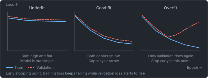
- The point where the validation loss hits bottom and rises again is the reference point for early stopping.
- If training and validation are both high and flat, you need to enlarge the model or train longer (underfitting).
Mitigating overfitting:
- More data, data augmentation
- Regularization (L1/L2), dropout
- Reduce model complexity, early stopping
- Reduce the number of features
Mitigating underfitting:
- Increase model complexity, train longer
- Add better features, relax regularization
A team trained an image classification model and got 99% training accuracy and 70% validation accuracy, a large gap. A classic overfit. After adding data augmentation (rotation, flip) and dropout and applying early stopping, the gap narrowed to 95% training / 91% validation and generalization improved. Lesson: the train-validation gap is the key signal of overfitting, and regularization, augmentation, and early stopping are the standard prescriptions.
Cross-Validation
If you split off the validation set only once, the evaluation wobbles depending on the luck of that split. k-fold cross-validation divides the data into k pieces, uses each piece once as validation and trains on the rest, and then averages the k performances. It gives a stable evaluation especially when data is scarce.
k=5 example:
Fold1: [valid][train][train][train][train]
Fold2: [train][valid][train][train][train]
...    → train/evaluate 5 times, then average
- Stratified k-fold: each fold keeps the class proportions — important for imbalanced classification.
- Time-series data: you must use a time-series split that validates on the future (keeping the past→future order) to prevent future leakage. Random k-fold is unsuitable for time series.
from sklearn.model_selection import StratifiedKFold, TimeSeriesSplit, cross_val_score

# Imbalanced classification: keep class proportions in each fold
cv = StratifiedKFold(n_splits=5, shuffle=True, random_state=42)
print(cross_val_score(model, X, y, cv=cv, scoring='f1').mean())

# Time series: always train on the past and validate on the future
tscv = TimeSeriesSplit(n_splits=5)
print(cross_val_score(model, X, y, cv=tscv, scoring='neg_root_mean_squared_error').mean())
The value of cross-validation lies in reducing the variance of the evaluation. A single train/test split is an estimate (high variance) that depends on the luck of that split. k-fold averages over several splits to lower the variance of the estimate, and uses the data for both training and validation, so it uses scarce data efficiently. But note that the larger k is, the more the training is repeated k times and the cost rises, and for order-meaningful data like time series, a random split leaks future information and inflates the evaluation.
Data Leakage That Quietly Ruins Evaluation
Most cases of "the validation score is great but it collapses in production" are not overfitting but leakage. It is the item to suspect even before metric selection.
| Symptom | Cause | Action |
|---|---|---|
| Validation accuracy is unrealistically high (0.99+) | Features derived from the answer are mixed in (target leakage) | Redefine feature creation time relative to the prediction time |
| Cross-validation is good but production performance drops sharply | The scaler/encoder was fit on the whole data first | fit only on the training fold after splitting, and only transform for validation |
| A time-series model fits well only in the backtest | Random k-fold put future data into training | Keep order with a time-series split |
| Records of the same customer/patient are split between training and validation | Group leakage | Split by group (the same entity goes to only one side) |
| Score jumps after oversampling | Oversampled even the validation set, so duplicate samples exist on both sides | Split → resample only the training set |
⚠️ Pitfall: Code that does preprocessing (normalization, missing-value imputation, encoding) on the whole data before splitting is easily used as a wrong choice on the exam. This is because distribution information from the validation set flows into training and the evaluation is inflated optimistically. The correct answer is always "split first, then fit the preprocessing on the training set and apply it to validation."
How to Choose
What is the problem type?
 ├─ Classification
 │    ├─ Balanced classes       → accuracy is also possible, F1 if needed
 │    └─ Imbalanced classes      → accuracy is off-limits
 │         ├─ Must not miss       → recall · AUC-PR
 │         ├─ False alarms costly → precision
 │         └─ Need balance        → F1  (+ fine-tune by adjusting the threshold)
 └─ Regression
      ├─ Large errors are fatal    → RMSE
      ├─ Many outliers             → MAE
      └─ Comparing explanatory power → R² (adjusted R² if the feature counts differ)

What is the evaluation procedure?
 ├─ Data is scarce             → k-fold  (imbalanced = stratified, time series = time-series split)
 ├─ Train-validation gap is large → overfitting → regularization · augmentation · early stopping
 └─ Score is unrealistically high → suspect leakage first
In the next lesson we review the whole of Week 5 — custom training, distributed training, debugging and profiling, and evaluation — together.
📖 Glossary
- Confusion matrix (TP / FP / FN / TN): A table that organizes prediction and actual into four cells by right/wrong, and every classification metric comes from here. The four cells are, respectively, positives correctly caught (TP), positives wrongly caught (FP, false alarms), positives missed (FN), and negatives correctly passed over (TN).
- Precision: "Of those flagged as positive, what percent are real." Look at it when you want to cut false alarms.
- Recall: "What percent of the actual positives were caught." Look at it when you must not miss anything.
- F1: The harmonic mean of precision and recall. The score does not rise easily if only one side is high.
- ROC-AUC / AUC-PR: ROC-AUC is the area under the curve drawn while varying the threshold and means overall discriminative power not tied to a threshold. AUC-PR is the area of the precision-recall curve, and is more honest than ROC-AUC when positives are very rare.
- Threshold: The boundary that cuts a probability into positive/negative. The default 0.5 is only a convention; it is an operating value you can adjust.
- Overfitting / underfitting: A state of memorizing the training data and collapsing on new data / a state of not having learned enough yet.
- Early stopping: Stopping training when validation performance starts to get worse.
- k-fold cross-validation: A method of dividing the data into k pieces, validating on each in turn, and averaging the results to stabilize the evaluation.
- Data leakage: A phenomenon in which information that should not be knowable at evaluation time gets mixed into training and inflates the score.
📝 Practice Questions
Click a choice to reveal the answer and explanation.
Question 1
You are evaluating a model on a highly imbalanced dataset in which fraudulent transactions are 1% of the total. Which of the following is the LEAST appropriate metric for judging model performance?
Question 2
In a cancer screening model, missing actual patients (false negatives) is the most dangerous. Which metric should be raised first?
Question 3
A model has 99% training accuracy but 70% validation accuracy, a large gap between the two. What are the diagnosis and the appropriate mitigation?
Question 4
In a regression model, you want to evaluate and optimize so as to avoid large errors by strongly penalizing rarely occurring large prediction errors. Which metric is appropriate?
Question 5
With little data, the evaluation from a single train/test split fluctuates greatly depending on the luck of the split. What is a method for stable evaluation?